Calculating point density for a UAV lidar survey
Sensor rate, altitude and ground speed to points per square meter.
A lidar spec sheet gives a rate per second. A survey plan needs points per square meter on the ground. The arithmetic between them fits on a napkin, and it goes wrong in two places: the pulses are counted as though they all reach bare ground, and the ground is treated as though it faces the sensor. Both errors push the answer the same way, so the estimate comes out high and the delivered survey falls short of it.
The sensor throughout is a GeoSLAM ZEB Horizon, which the lab flies on a DJI Matrice M600.
Pulses, returns, and ground returns
The word “points” is used for three different quantities.
- Emitted pulses.
- What the sensor fires. The only one of the three that is set by the instrument alone.
- Returns.
- What lands in the file. One pulse can produce several returns or none, and points divided by run duration gives a delivered rate.
- Ground returns.
- The subset that came off bare ground, with canopy, water and wire returns excluded. What a DEM is built from, and always the smallest of the three.
The manual’s specification table calls this sensor’s figure a scan rate and states it in points per second: 300,000. That unit names the second quantity, not the first, and the formulas below want the first. The lab’s own unit has an operator-confirmed emitted rate of 288,000 per second, four percent lower. This page still uses 300,000 as R, so its results can be set beside the lab’s derivation, which does the same.
Every formula on this page counts emitted rays, so each result is an idealized count of ray-ground intersections rather than of returns. It is not a bound on either of the other two quantities: a single pulse through a canopy can return several times.
Instantaneous density on the ground
Points per second per square meter at lateral distance x from nadir, under a sensor at height h firing at rate R.
N(x) = R h / [ 4π (h2 + x2)3/2 ]
The pulses spread over a sphere, which costs the familiar inverse square. They then land on ground that is horizontal while the ray reaching it is oblique, and that stretches every footprint by 1 / cos θ, with cos θ = h / (h2 + x2)1/2.
Dropping the projection gives density on a sphere, not on the ground. The error is zero at nadir and grows outward: it overstates density by 1.41× one altitude out from nadir, 2.24× two altitudes out, and an accumulated single-pass estimate by 1.21×, giving 200 points per square meter where the corrected form gives 165 under the conditions worked below.
As a ratio to the nadir value, the falloff has no instrument in it:
N(x) / N0 = (1 + x2 / h2)−3/2
So one altitude out from nadir the ground gets 0.354 of the nadir rate, and two altitudes out 0.089. At nadir the rate itself is R / (4πh2), which at 50 m AGL is 9.5 points per second per square meter.
What the 4π is doing
The 4π divides the emitted rate evenly over a whole sphere, and the ZEB Horizon does not: it sweeps 360° by 270°, about 85 percent of the solid angle, and concentrates its points along a rotating fan. The 4π is a normalization convention, not a measured property of the instrument. Fitting this model to one of the lab’s own handheld clouds put the free scale factor at 1.264 — above one, which a true physical normalization could not be. Within this model geometry sets the shape of the falloff and the level is a convention that a fit against real data can move. A real rotating fan need not respect even that much: an angular distribution that is not isotropic changes the shape as well.
Where the swath ends
Two boundaries, and which one binds depends on altitude.
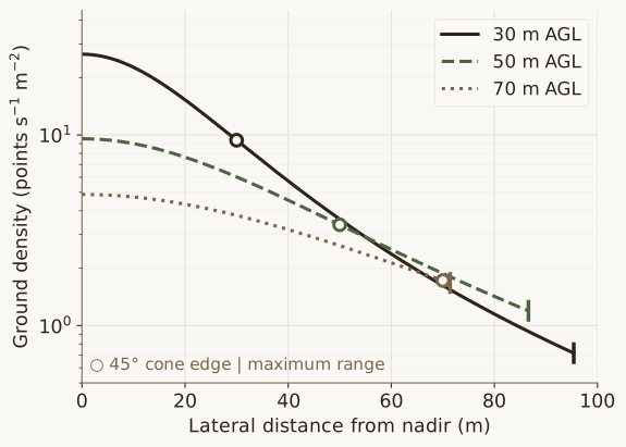
A 45° half-angle cone has a ground radius equal to the altitude, so its full swath is 2h — 100 m at 50 m AGL. Maximum sensor range, roughly 100 m for this instrument in favorable conditions, gives a ground radius of (r2 − h2)1/2 instead, which at 50 m AGL is 86.6 m. The two are equal at h = r / √2, or 70.7 m. Above that the cone is wider than the sensor can reach and range sets the swath.
Five things get called the swath, and only the first two are set by the instrument. Maximum sensor range, about 100 m here. Geometric swath, where returns are physically possible, which is whatever that range reaches: 173 m total at 50 m AGL. The 45° cone, a planning convention rather than a limit, which at that altitude is narrower — 100 m total — and is the figure the lab’s envelope quotes. High-quality swath, the middle where density and incidence are acceptable, which that envelope puts at 50 to 60 m. Flight-line spacing, which the flight plan sets rather than the sensor: for detailed work the lab plans lines at 25 to 30 m.
Density accumulated along a pass
N(x) is a rate. A survey delivers the integral of it.
As the aircraft approaches a fixed point on the centerline, that point’s lateral distance from nadir falls to zero and rises again, so integrating N along the track gives accumulated density there. Write along-track distance as s, which on the centerline is the same thing as x, and integrate from −L to +L, divided by ground speed v:
PDcenterline = R / (2π h v) × L / (h2 + L2)1/2
The sensor sets L, not the planner. A round 100 m is the tempting limit and it is the wrong one: at 50 m AGL a ground point 100 m along the track sits at a slant range of 111.8 m, past the instrument’s 100 m reach, so integrating that far counts ground the sensor could not range. Stopping where the ground leaves the range sphere puts L = (r2 − h2)1/2 = 86.6 m and the tail factor at (1 − h2/r2)1/2 = 0.866. At R = 300,000 per second and h = 50 m the prefactor is then 827 / v: centerline density is inversely proportional to ground speed. The spacing column is the nominal 1 / √PD, the spacing a uniform square grid of that density would have.
| Ground speed (m/s) | Centerline (pts/m²) | Spacing (cm) |
|---|---|---|
| 1 | 827 | 3.5 |
| 3 | 276 | 6.0 |
| 5 | 165 | 7.8 |
| 6 | 138 | 8.5 |
| 8 | 103 | 9.8 |
| 10 | 83 | 11.0 |
Off the centerline the same integral applies at cross-track offset y. The ground point’s distance from nadir is (s2 + y2)1/2 throughout the pass, and the range sphere closes the along-track window to (r2 − h2 − y2)1/2:
PD(y) = R h L / [ 2π (h2 + y2) (h2 + y2 + L2)1/2 v ]
At 50 m to the side of a line flown at 50 m AGL and 5 m/s that gives 67 points per square meter, 41 percent of the centerline value. It is tempting to skip the integral and scale the centerline figure by the instantaneous ratio N(y) / N0, which is 0.354 at that offset. That gives 58, and it is the wrong operation: the instantaneous ratio compares two points at one instant, while moving off the centerline shifts the whole along-track profile rather than only its peak.
Halving speed doubles density on one pass and halves the ground covered, so density and coverage trade against each other. Flown twice over one line at 6 m/s, a strip ends with the 276 points per square meter that a single pass at 3 m/s would have given it, and the SLAM solution gets a second look at the same ground. Flown once over each of two adjacent lines at 6 m/s, the same flying time covers twice the ground at 138. The lab’s planning envelope calls for 5 to 6 m/s with repeat passes.
A worked example at 50 m and 5 m per second
A spec-sheet example, not a flight: R and r are the sensor’s stated figures, and the altitude and speed are the lab’s planning values.
given   R = 300,000 /s            sensor rate, spec sheet
        h = 50 m                  altitude, planning value
        v = 5 m/s                 ground speed, planning value
        r = 100 m                 maximum range, which sets
                                  both limits below

nadir   N0 = R / (4 pi h^2)
           = 300,000 / (4 pi x 2,500)        =    9.5 /s/m^2

pass    L = (r^2 - h^2)^0.5                  =   86.6 m
        PD = R / (2 pi h v) x L / (h^2+L^2)^0.5
           = 954.9 x 0.866 / 5               =    165 pts/m^2
        spacing = 1 / sqrt(165)              =    7.8 cm

edge    y = 50 m to the side, so L falls to
        (r^2 - h^2 - y^2)^0.5                =   70.7 m
        PD(y) = R h L / [2 pi (h^2+y^2)
                 x (h^2+y^2+L^2)^0.5 x v]    =     67 pts/m^2

ground  new ground per pass = line spacing x speed
        25 m x 5 m/s = 125 m^2/s             =   0.75 ha/min
Every figure there is per pass, counted in emitted rays. Overlapping lines add; the lab’s derivation covers a single pass and supplies no overlap factor.
What one of the lab’s flights delivered
ZEB Horizon flown at Tisch Park, 19 April 2024. Measured from the processed cloud.
1,016 s
on task
3.59 m/s
median ground speed
77,596/s
delivered rate
22.0 acres
covered
The delivered rate is 26 percent of the spec rate, and those are returns of every kind at every height, well short of ground returns. Spread over the 89,193 square meters covered, the 78,837,683 points average 884 per square meter.
The altitude flown is not recorded alongside that cloud, so the run cannot test N(x) directly.
The same sensor carried by hand delivered 120,993 per second over mown parkland at Tisch Park in May 2025 and 86,613 per second over broken outcrop at Donze Farm in December 2023: one instrument and one spec rate, with delivered rates 40 percent apart. Delivered rate depends on the run at least as much as on the sensor — on what the beam met, and on how the cloud was processed.
Sanity check
Integrating N over the whole ground plane returns exactly R / 2, so within this model a pass puts no more than 150,000 points per second on the ground however the swath is arranged. Across a swath of width W advancing at speed v, the average density then cannot exceed R / (2Wv): over the 45° cone’s 100 m at 5 m/s, 300 points per square meter. That half is a property of the 4π convention, not a bound on the instrument — a downward-looking sensor can point far more than half its rays at the ground — so it catches arithmetic that contradicts the model it came from, not physics.
UAV lidar at the lab
The lab plans, flies and processes UAV and terrestrial lidar surveys, and sizes them to the density the target needs.