How point density falls off with distance from a laser scanner
The angular grid, the grazing cosine, and what occlusion adds, with numbers from two of the lab's survey-planning studies.
Set a scanner up in a cemetery and two surfaces in the same frame thin out at different rates. The face of a headstone 20 m away is still densely sampled while the grass in front of it has gone sparse — both surfaces at the same range, in one scan, from one instrument. The difference is the angle each surface makes with the ray, and that angle costs a whole power of distance.
The numbers below come from two of the lab's survey-planning studies, which rest on the same geometry. One is open ground at Greenwood Cemetery, where the sampling grid is projected onto a flat surface and obstacles are left out deliberately. The other is forest at Tyson Research Center, where the falloff is fitted to a cloud the lab had already collected, so obstacles sit inside the fit.
The angular grid and the 1/r² law
A scanner sweeps a regular grid of directions, spaced by some small angle δ, and fires along each one. At range r two adjacent directions land r·δ apart, so each sample owns a patch of about (rδ)², and the areal density on a surface perpendicular to the beam is
ρ(r) = 1 / (r² · δ²)
The law carries no free parameter, and both studies take it as given. At the SX12's fitted angular spacing of 1.274 mrad, a wall 20 m from the instrument receives about 1,540 points/m² — ground at that range does much worse.
Projecting the grid onto the ground
A ray leaving a tripod at height h and landing at horizontal distance d arrives at grazing incidence, so the cosine between the ray and the ground normal is h/r. Carrying that factor through gives the density on locally planar ground as
ρ(d) = h / ((d² + h²)3/2 · δ²)
Far from the instrument the h² term stops mattering and this reduces to h / (d³ · δ²), so ground density falls as the cube of distance, not the square.
The ratio between a facing surface and the ground at the same range is then about d/h, which at 20 m from a 1.5 m tripod puts the headstone at roughly 13 times the grass. Once d is well past h, ground density scales linearly with instrument height, so a taller tripod lifts the returns out where these examples sit.
A datasheet quotes point spacing at a stated range, such as the SX12's coarse mode at 50 mm at 50 m. That is the spacing on a target perpendicular to the beam — read as a ground density it is wrong by the same factor of d/h, and a survey planned on it comes out short of setups.
Nominal and effective angular spacing
The δ in both formulas is the angular grid the instrument was set to, the nominal spacing, but real ground does not return one point per emitted ray. Fitting the ground law to the lab's own scans therefore recovers a spacing coarser than the one dialed in — the effective spacing, and the one a plan should be built on.
| Instrument | Nominal | Effective, fitted | Fit window |
|---|---|---|---|
| Trimble SX12 | 1.00 mrad | 1.274 mrad | 3–56 m |
| Trimble X9 | not recorded | 0.577 mrad | 3–40 m |
Fitted on mown parkland and on a tree scan. The height is not a measured setup height: 1.5, 1.6 and 1.8 m were each tried and 1.5 m left the smallest residual. The X9's scan mode is absent from its export, so its nominal spacing is unknown.
An SX12 set to 1.00 mrad behaves like 1.274 mrad on mown grass. The share of the ideal grid that ground actually returns is (δnominal / δeffective)² = 0.616, so a plan built on the brochure number overstates density by about 1.6×. The error in setups is smaller, because the two quantities scale differently: ground density goes as the cube of station spacing and stations per unit area as its square. Recovering a factor of 1.62 in density needs the spacing to close by 1.18, which raises the station count by 1.38×.
Occlusion, and what a fitted kernel adds
Obstacles play no part in either formula so far. The Greenwood study leaves it out as a scoping decision and calls it the study's largest omission: a cemetery is a field of vertical opaque objects about as tall as the tripod, which is the worst geometry there is for a grazing ground ray. In forest the omission becomes the largest term in the problem, so the Tyson planning kept the 1/r² geometry and fitted the remainder to a cloud the lab had already collected.
k(r) = C · (r + 0.5)−2 · exp(−(r/L)p)
The exponent on the geometric term is held at 2, so only the envelope is fitted. On a three-station SX12 scan of the ForestGEO plot, 24.0 million points from stations about 22 m apart, the envelope comes back at L ≈ 14 m and p ≈ 0.84. Rescaled so one station integrates to the observed 8.0 million points, it accounts for 98 % of the plot's point total — a check on totals, not a measure of how closely it tracks any one cell.
The exponential term models no particular physical process; it is a measured envelope that folds the grazing projection and the shadowing by stems into a single quantity. About 85 % of a scan's points land within 10 m of the instrument and 96 % within 25 m, both read off the cloud rather than off the kernel, and density stays above the forest plan's threshold of 5 points/m² out to roughly 60 m.
| Density target (points/m²) | Reached out to (m) |
|---|---|
| 100 | 30 |
| 50 | 36 |
| 20 | 45 |
| 10 | 53 |
| 5 | 61 |
| 1 | 83 |
One 15-minute SX12 scan in deciduous forest, all returns.
Density against range for three surfaces
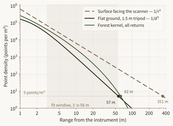
The three curves do not all use the same parameters. The facing-surface and flat-ground curves both use the SX12's fitted 1.274 mrad, and the shaded band is the range interval the ground law was fitted over; outside it that curve is an extrapolation. The forest curve carries no angular spacing at all. It is the Tyson kernel, its normalization recovered from that study's own per-station total of 8.0 million points, and it reproduces the study's published useful-radius table to within about a meter at every row. The reference line at 5 points/m² is the sparse-coverage threshold from the forest plan.
The facing-surface line is straight at a slope of −2 and crosses 5 points/m² only at 351 m, which is about as far as the instrument ranges at all: the SX12 datasheet gives 0.9 to 350 m against a Kodak gray card and 0.9 to 600 m against a white one, so on a dark target the sampling geometry and the ranging give out together. Flat ground steepens toward −3 and crosses at 57 m. The forest kernel begins near −2.5 at 10 m and steepens through −3.6 at 30 m to −4.8 at 60 m, so density in forest falls away far faster than it does on a lawn.
Worked example: SX12 station spacing on open ground
Take a target of 100 points/m², a 10 cm ground sample spacing, over open mown ground, with the SX12 on a 1.5 m tripod at its fitted 1.274 mrad. Solving the ground law for that target puts a single station's useful radius at 20.9 m. Treating the radius as a coverage disc and packing the stations so the discs just touch undercounts badly, because density from separate stations adds.
On a triangular lattice, which is the fewest setups for a given worst-case range, the worst-served ground sits at the circumradius of a triangle, s/√3 from each of its three stations. At a spacing of s = 48 m that worst point is 27.7 m from three stations. One station delivers 43 points/m² there and three deliver 130, so the target is met at more than twice the spacing the single-station radius suggested.
The full planning run for that scenario, using a 2 m raster, a spacing sweep and the real parcel outline, settles on the same 48 m spacing. The lattice it solves is 67 stations, covering 93.3 % of the footprint at or above target with a 10th-percentile density of 127 points/m²; the study then reports 81 after adding its 20 % margin for obstructions, access and re-setups, which the coverage figures do not include. The arithmetic above lands within about 3 % of the modeled density.
A scanner that moves along a track
A handheld or vehicle-mounted scanner obeys the same grazing geometry, but the sensor moves. Density accumulated at a point is then an integral of the instantaneous rate along the track, not a fixed dwell from one position. That integral returns one power of distance: ground density falls as 1/x² with offset from a walked line, against 1/d³ from a station. The clean 1/x² holds for a straight track long compared with the offset, walked at constant height and speed, with nothing attenuating the returns — conditions the fit below then relaxes.
The instantaneous rate keeps the same h/r³ shape, with the delivered point rate R standing where 1/δ² stands in the static case: N(x) = R·h / (4π (h² + x²)3/2) points per second per square meter. That expression is the geometry alone. What is fitted sits on top of it: an attenuation factor exp(−(d/L)p) standing for range gating, field of view and obstruction, and a realization factor absorbing the 4π convention. Fitted to a GeoSLAM ZEB Horizon walk over mown parkland at 0.82 m/s, with a 1.38 m sensor height read from the trajectory file and 120,993 points/s delivered, it returns L = 26 m, p = 5.4 and a realization factor of 1.26, over a validated window of 2 to 16 m.
Delivered is not the same as emitted. The sensor emits 288,000 points/s, while the two calibration walks delivered 120,993 and 86,613 points/s, and the delivered rate is the one that predicts delivered density. A plan built on the emitted figure is off by more than a factor of two before any geometry has been applied.
Sanity checks
- Ground density should drop by about 1000× when range goes up 10×. Grazing ground, stems, brush and terrain steepen it.
- Compare like surfaces only. An all-return density in forest and a ground-only density on a lawn are different quantities, however similar the units look.
The forest cloud behind the fitted kernel is public: the merged three-station ForestGEO SX12 scan of 2026-05-14, 24.0 million points, EPSG:6512+5703, as COPC (189 MB, spatially indexed, so a reader can range-request one part of it).
Terrestrial laser scanning at the lab
The lab runs tripod and handheld laser scanning, plans station layouts against measured density, and registers and publishes the resulting clouds.